Hypothesis Testing

To learn more about hypothesis testing. And for quiz 13.

library(tidyverse)
library(infer)
library(moderndive)
library(nycflights13)
library(ggplot2movies)

promotions %>% 
  sample_n(size = 6) %>% 
  arrange(id)

# A tibble: 6 x 3
     id decision gender
  <int> <fct>    <fct> 
1     2 promoted male  
2     8 promoted male  
3    22 promoted female
4    35 promoted female
5    40 not      female
6    46 not      female

ggplot(promotions, aes(x = gender, fill = decision)) +
  geom_bar() +
  labs(x = "Gender of name on résumé")

promotions %>% 
  group_by(gender, decision) %>% 
  tally()

# A tibble: 4 x 3
# Groups:   gender [2]
  gender decision     n
  <fct>  <fct>    <int>
1 male   not          3
2 male   promoted    21
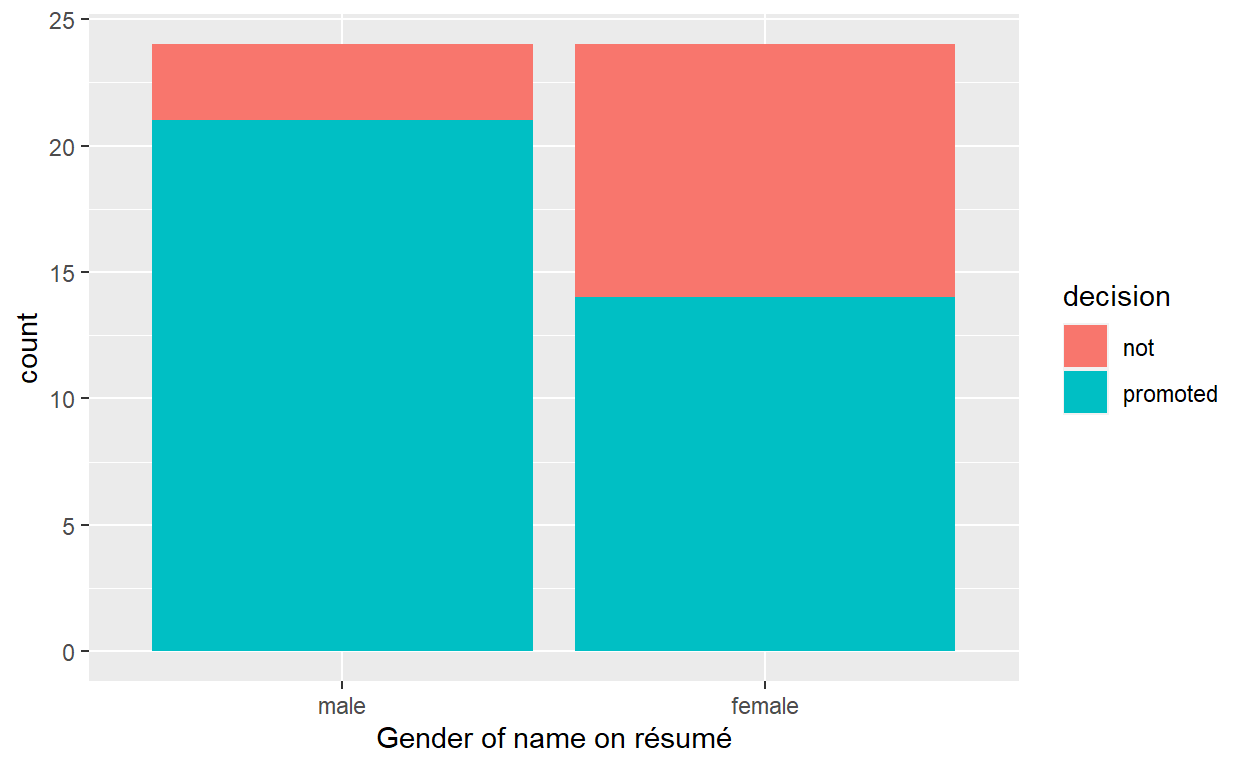
3 female not         10
4 female promoted    14

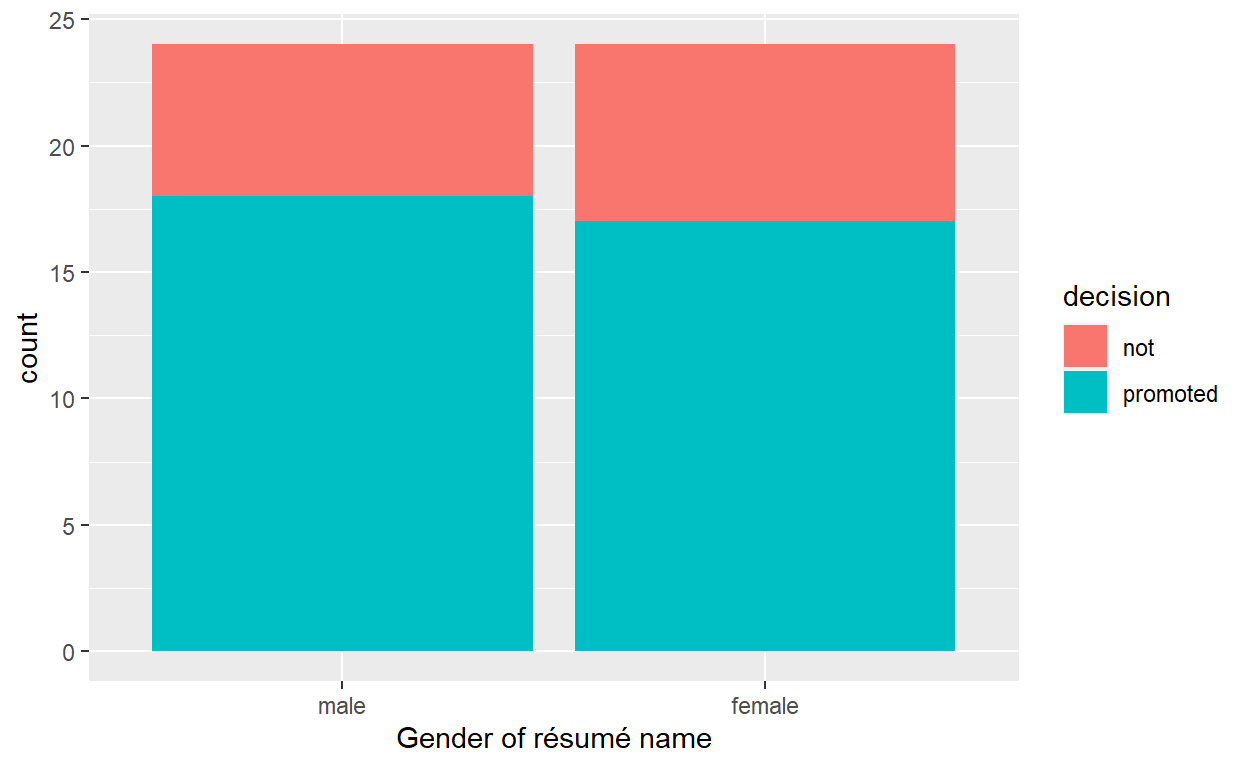
ggplot(promotions_shuffled, 
       aes(x = gender, fill = decision)) +
  geom_bar() + 
  labs(x = "Gender of résumé name")

promotions_shuffled %>% 
  group_by(gender, decision) %>% 
  tally() # Same as summarize(n = n())

# A tibble: 4 x 3
# Groups:   gender [2]
  gender decision     n
  <fct>  <fct>    <int>
1 male   not          6
2 male   promoted    18
3 female not          7
4 female promoted    17

promotions %>% 
  specify(formula = decision ~ gender, success = "promoted") 

Response: decision (factor)
Explanatory: gender (factor)
# A tibble: 48 x 2
   decision gender
   <fct>    <fct> 
 1 promoted male  
 2 promoted male  
 3 promoted male  
 4 promoted male  
 5 promoted male  
 6 promoted male  
 7 promoted male  
 8 promoted male  
 9 promoted male  
10 promoted male  
# ... with 38 more rows

promotions %>% 
  specify(formula = decision ~ gender, success = "promoted") %>% 
  hypothesize(null = "independence")

Response: decision (factor)
Explanatory: gender (factor)
Null Hypothesis: independence
# A tibble: 48 x 2
   decision gender
   <fct>    <fct> 
 1 promoted male  
 2 promoted male  
 3 promoted male  
 4 promoted male  
 5 promoted male  
 6 promoted male  
 7 promoted male  
 8 promoted male  
 9 promoted male  
10 promoted male  
# ... with 38 more rows

promotions_generate <- promotions %>% 
  specify(formula = decision ~ gender, success = "promoted") %>% 
  hypothesize(null = "independence") %>% 
  generate(reps = 1000, type = "permute")
nrow(promotions_generate)

[1] 48000

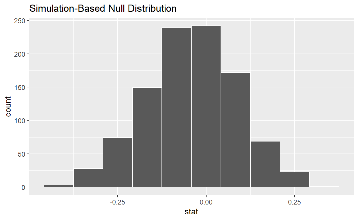
null_distribution <- promotions %>% 
  specify(formula = decision ~ gender, success = "promoted") %>% 
  hypothesize(null = "independence") %>% 
  generate(reps = 1000, type = "permute") %>% 
  calculate(stat = "diff in props", order = c("male", "female"))
null_distribution

Response: decision (factor)
Explanatory: gender (factor)
Null Hypothesis: independence
# A tibble: 1,000 x 2
   replicate    stat
       <int>   <dbl>
 1         1  0.0417
 2         2 -0.292 
 3         3  0.0417
 4         4 -0.125 
 5         5  0.125 
 6         6  0.0417
 7         7  0.125 
 8         8  0.0417
 9         9  0.125 
10        10  0.0417
# ... with 990 more rows

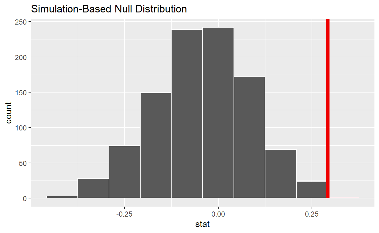
obs_diff_prop <- promotions %>% 
  specify(decision ~ gender, success = "promoted") %>% 
  calculate(stat = "diff in props", order = c("male", "female"))
obs_diff_prop

Response: decision (factor)
Explanatory: gender (factor)
# A tibble: 1 x 1
   stat
  <dbl>
1 0.292

visualize(null_distribution, bins = 10)

visualize(null_distribution, bins = 10) + 
  shade_p_value(obs_stat = obs_diff_prop, direction = "right")

null_distribution %>% 
  get_p_value(obs_stat = obs_diff_prop, direction = "right")

# A tibble: 1 x 1
  p_value
    <dbl>
1   0.024

null_distribution <- promotions %>% 
  specify(formula = decision ~ gender, success = "promoted") %>% 
  hypothesize(null = "independence") %>% 
  generate(reps = 1000, type = "permute") %>% 
  calculate(stat = "diff in props", order = c("male", "female"))

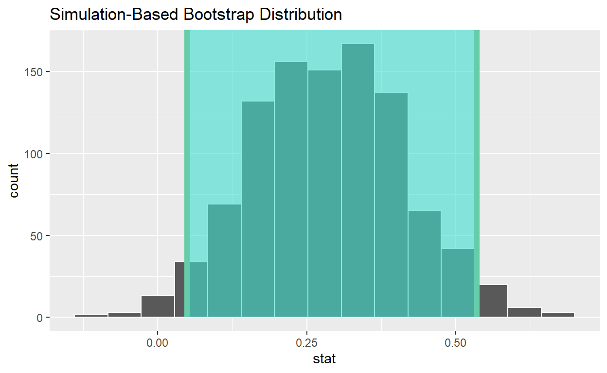
bootstrap_distribution <- promotions %>% 
  specify(formula = decision ~ gender, success = "promoted") %>% 
  # Change 1 - Remove hypothesize():
  # hypothesize(null = "independence") %>% 
  # Change 2 - Switch type from "permute" to "bootstrap":
  generate(reps = 1000, type = "bootstrap") %>% 
  calculate(stat = "diff in props", order = c("male", "female"))

percentile_ci <- bootstrap_distribution %>% 
  get_confidence_interval(level = 0.95, type = "percentile")
percentile_ci

# A tibble: 1 x 2
  lower_ci upper_ci
     <dbl>    <dbl>
1   0.0489    0.534

visualize(bootstrap_distribution) + 
  shade_confidence_interval(endpoints = percentile_ci)

se_ci <- bootstrap_distribution %>% 
  get_confidence_interval(level = 0.95, type = "se", 
                          point_estimate = obs_diff_prop)
se_ci

# A tibble: 1 x 2
  lower_ci upper_ci
     <dbl>    <dbl>
1   0.0447    0.539

visualize(bootstrap_distribution) + 
  shade_confidence_interval(endpoints = se_ci)

movies

# A tibble: 58,788 x 24
   title       year length budget rating votes    r1    r2    r3    r4
   <chr>      <int>  <int>  <int>  <dbl> <int> <dbl> <dbl> <dbl> <dbl>
 1 $           1971    121     NA    6.4   348   4.5   4.5   4.5   4.5
 2 $1000 a T~  1939     71     NA    6      20   0    14.5   4.5  24.5
 3 $21 a Day~  1941      7     NA    8.2     5   0     0     0     0  
 4 $40,000     1996     70     NA    8.2     6  14.5   0     0     0  
 5 $50,000 C~  1975     71     NA    3.4    17  24.5   4.5   0    14.5
 6 $pent       2000     91     NA    4.3    45   4.5   4.5   4.5  14.5
 7 $windle     2002     93     NA    5.3   200   4.5   0     4.5   4.5
 8 '15'        2002     25     NA    6.7    24   4.5   4.5   4.5   4.5
 9 '38         1987     97     NA    6.6    18   4.5   4.5   4.5   0  
10 '49-'17     1917     61     NA    6      51   4.5   0     4.5   4.5
# ... with 58,778 more rows, and 14 more variables: r5 <dbl>,
#   r6 <dbl>, r7 <dbl>, r8 <dbl>, r9 <dbl>, r10 <dbl>, mpaa <chr>,
#   Action <int>, Animation <int>, Comedy <int>, Drama <int>,
#   Documentary <int>, Romance <int>, Short <int>

movies_sample

# A tibble: 68 x 4
   title                     year rating genre  
   <chr>                    <int>  <dbl> <chr>  
 1 Underworld                1985    3.1 Action 
 2 Love Affair               1932    6.3 Romance
 3 Junglee                   1961    6.8 Romance
 4 Eversmile, New Jersey     1989    5   Romance
 5 Search and Destroy        1979    4   Action 
 6 Secreto de Romelia, El    1988    4.9 Romance
 7 Amants du Pont-Neuf, Les  1991    7.4 Romance
 8 Illicit Dreams            1995    3.5 Action 
 9 Kabhi Kabhie              1976    7.7 Romance
10 Electric Horseman, The    1979    5.8 Romance
# ... with 58 more rows

ggplot(data = movies_sample, aes(x = genre, y = rating)) +
  geom_boxplot() +
  labs(y = "IMDb rating")

movies_sample %>% 
  group_by(genre) %>% 
  summarize(n = n(), mean_rating = mean(rating), std_dev = sd(rating))

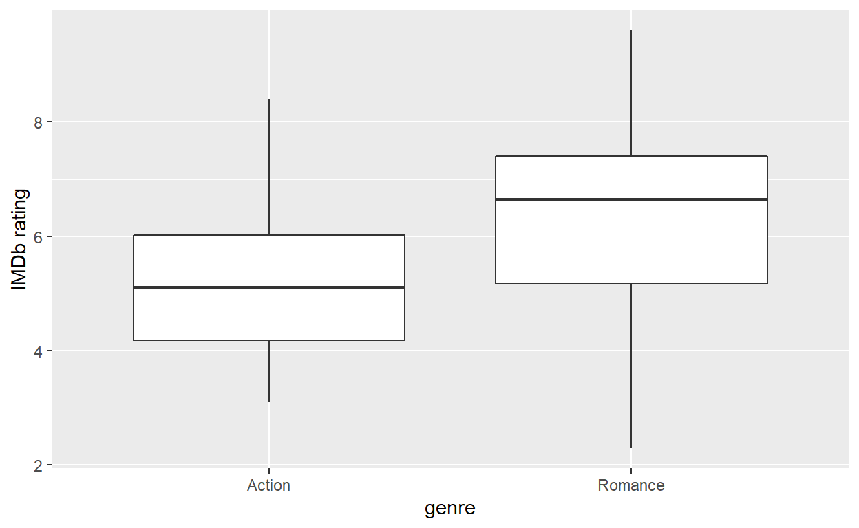
# A tibble: 2 x 4
  genre       n mean_rating std_dev
  <chr>   <int>       <dbl>   <dbl>
1 Action     32        5.28    1.36
2 Romance    36        6.32    1.61

movies_sample %>% 
  specify(formula = rating ~ genre)

Response: rating (numeric)
Explanatory: genre (factor)
# A tibble: 68 x 2
   rating genre  
    <dbl> <fct>  
 1    3.1 Action 
 2    6.3 Romance
 3    6.8 Romance
 4    5   Romance
 5    4   Action 
 6    4.9 Romance
 7    7.4 Romance
 8    3.5 Action 
 9    7.7 Romance
10    5.8 Romance
# ... with 58 more rows

movies_sample %>% 
  specify(formula = rating ~ genre) %>% 
  hypothesize(null = "independence")

Response: rating (numeric)
Explanatory: genre (factor)
Null Hypothesis: independence
# A tibble: 68 x 2
   rating genre  
    <dbl> <fct>  
 1    3.1 Action 
 2    6.3 Romance
 3    6.8 Romance
 4    5   Romance
 5    4   Action 
 6    4.9 Romance
 7    7.4 Romance
 8    3.5 Action 
 9    7.7 Romance
10    5.8 Romance
# ... with 58 more rows

movies_sample %>% 
  specify(formula = rating ~ genre) %>% 
  hypothesize(null = "independence") %>% 
  generate(reps = 1000, type = "permute") %>% 
  View()

null_distribution_movies <- movies_sample %>% 
  specify(formula = rating ~ genre) %>% 
  hypothesize(null = "independence") %>% 
  generate(reps = 1000, type = "permute") %>% 
  calculate(stat = "diff in means", order = c("Action", "Romance"))
null_distribution_movies

Response: rating (numeric)
Explanatory: genre (factor)
Null Hypothesis: independence
# A tibble: 1,000 x 2
   replicate    stat
       <int>   <dbl>
 1         1 -0.605 
 2         2 -0.339 
 3         3 -1.27  
 4         4  0.275 
 5         5  0.499 
 6         6 -0.132 
 7         7 -0.0201
 8         8  0.446 
 9         9  0.582 
10        10 -0.250 
# ... with 990 more rows

obs_diff_means <- movies_sample %>% 
  specify(formula = rating ~ genre) %>% 
  calculate(stat = "diff in means", order = c("Action", "Romance"))
obs_diff_means

Response: rating (numeric)
Explanatory: genre (factor)
# A tibble: 1 x 1
   stat
  <dbl>
1 -1.05

visualize(null_distribution_movies, bins = 10) + 
  shade_p_value(obs_stat = obs_diff_means, direction = "both")

null_distribution_movies %>% 
  get_p_value(obs_stat = obs_diff_means, direction = "both")

# A tibble: 1 x 1
  p_value
    <dbl>
1   0.008

movies_sample %>% 
  group_by(genre) %>% 
  summarize(n = n(), mean_rating = mean(rating), std_dev = sd(rating))

# A tibble: 2 x 4
  genre       n mean_rating std_dev
  <chr>   <int>       <dbl>   <dbl>
1 Action     32        5.28    1.36
2 Romance    36        6.32    1.61

Construct null distribution of xbar_a - xbar_r:

null_distribution_movies <- movies_sample %>% 
  specify(formula = rating ~ genre) %>% 
  hypothesize(null = "independence") %>% 
  generate(reps = 1000, type = "permute") %>% 
  calculate(stat = "diff in means", order = c("Action", "Romance"))
visualize(null_distribution_movies, bins = 10)

Construct null distribution of t:

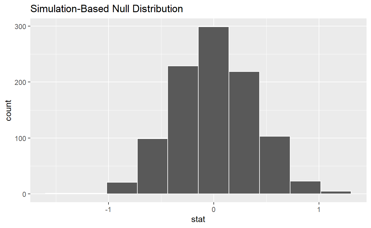
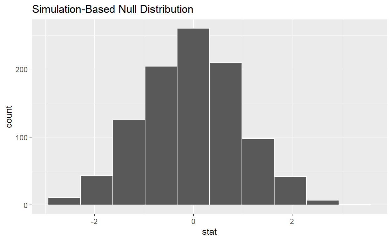
null_distribution_movies_t <- movies_sample %>% 
  specify(formula = rating ~ genre) %>% 
  hypothesize(null = "independence") %>% 
  generate(reps = 1000, type = "permute") %>% 
  # Notice we switched stat from "diff in means" to "t"
  calculate(stat = "t", order = c("Action", "Romance"))
visualize(null_distribution_movies_t, bins = 10)

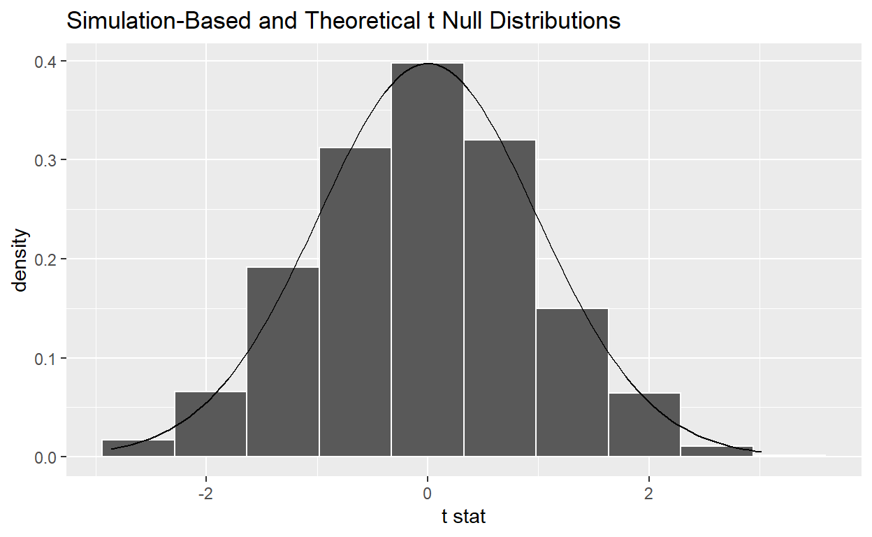
visualize(null_distribution_movies_t, bins = 10, method = "both")

obs_two_sample_t <- movies_sample %>% 
  specify(formula = rating ~ genre) %>% 
  calculate(stat = "t", order = c("Action", "Romance"))
obs_two_sample_t

Response: rating (numeric)
Explanatory: genre (factor)
# A tibble: 1 x 1
   stat
  <dbl>
1 -2.91

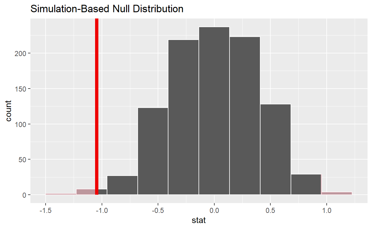
visualize(null_distribution_movies_t, method = "both") +
  shade_p_value(obs_stat = obs_two_sample_t, direction = "both")

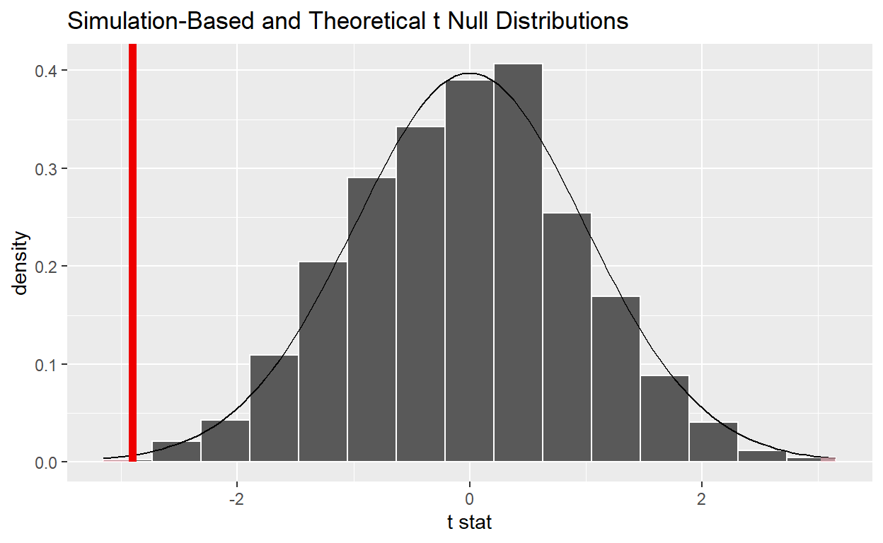
null_distribution_movies_t %>% 
  get_p_value(obs_stat = obs_two_sample_t, direction = "both")

# A tibble: 1 x 1
  p_value
    <dbl>
1       0

flights_sample <- flights %>% 
  filter(carrier %in% c("HA", "AS"))

ggplot(data = flights_sample, mapping = aes(x = carrier, y = air_time)) +
  geom_boxplot() +
  labs(x = "Carrier", y = "Air Time")

flights_sample %>% 
  group_by(carrier, dest) %>% 
  summarize(n = n(), mean_time = mean(air_time, na.rm = TRUE))

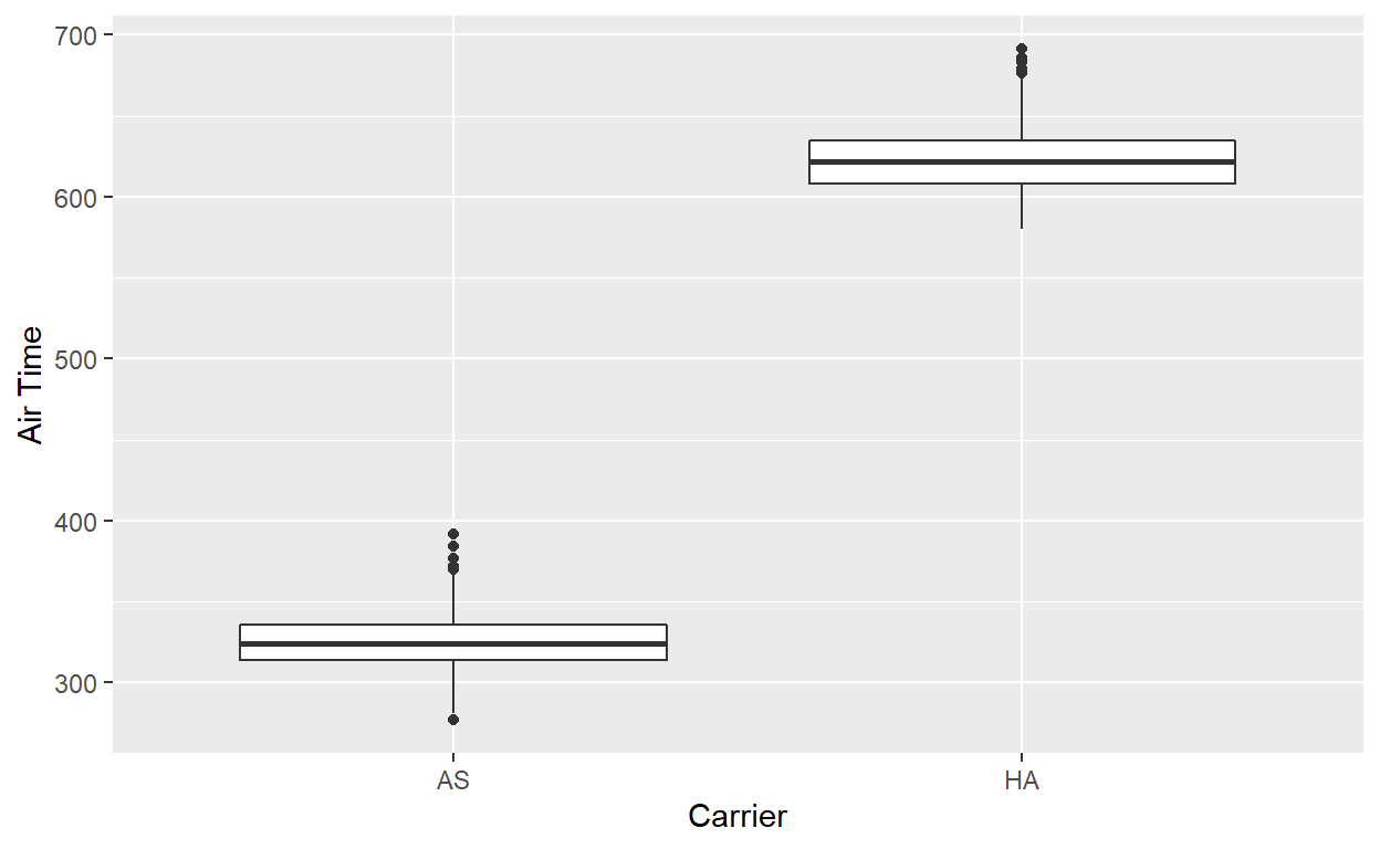
# A tibble: 2 x 4
# Groups:   carrier [2]
  carrier dest      n mean_time
  <chr>   <chr> <int>     <dbl>
1 AS      SEA     714      326.
2 HA      HNL     342      623.

Fit regression model:

score_model <- lm(score ~ bty_avg, data = evals)

Get regression table:

get_regression_table(score_model)

# A tibble: 2 x 7
  term      estimate std_error statistic p_value lower_ci upper_ci
  <chr>        <dbl>     <dbl>     <dbl>   <dbl>    <dbl>    <dbl>
1 intercept    3.88      0.076     51.0        0    3.73     4.03 
2 bty_avg      0.067     0.016      4.09       0    0.035    0.099