library(tidyverse)
library(moderndive)
library(infer)

moderndive::pennies_sample

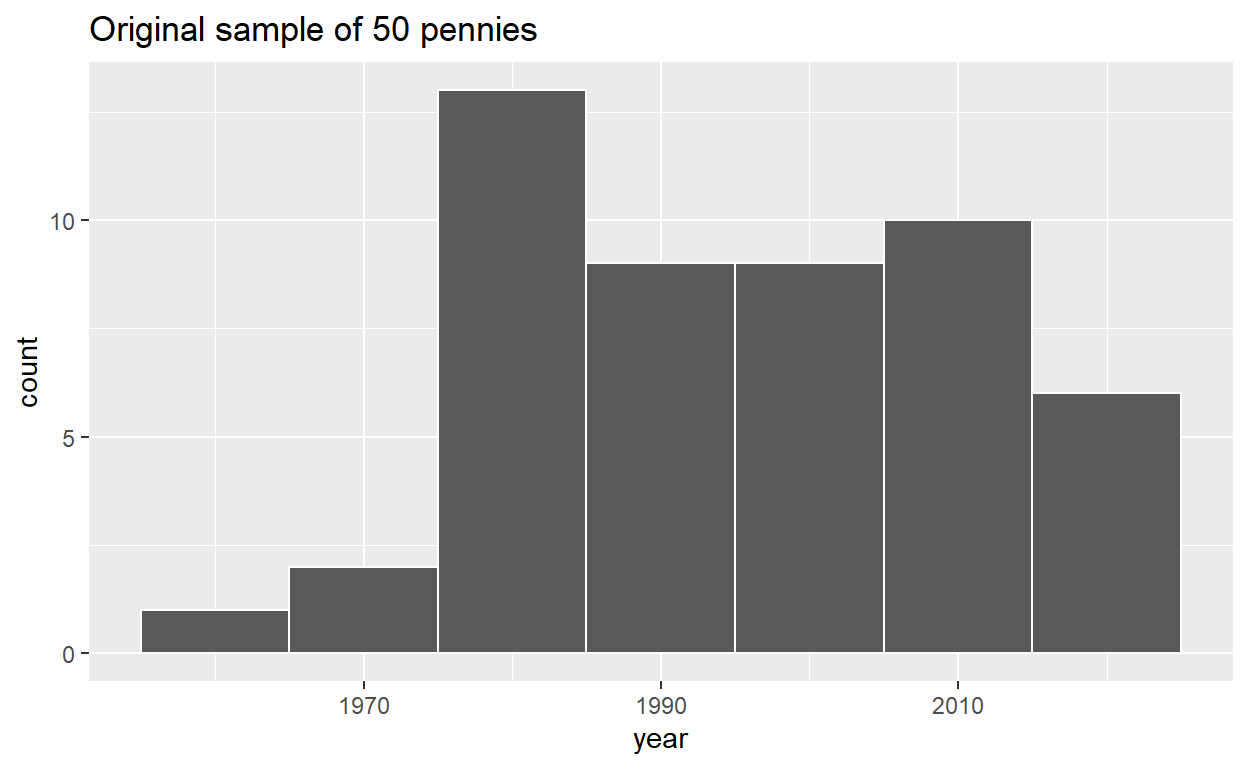
# A tibble: 50 x 2
      ID  year
   <int> <dbl>
 1     1  2002
 2     2  1986
 3     3  2017
 4     4  1988
 5     5  2008
 6     6  1983
 7     7  2008
 8     8  1996
 9     9  2004
10    10  2000
# ... with 40 more rows

ggplot(pennies_sample, aes(x = year)) +
  geom_histogram(binwidth = 10, color = "white")

x_bar <- pennies_sample %>% 
  summarize(mean_year = mean(year))

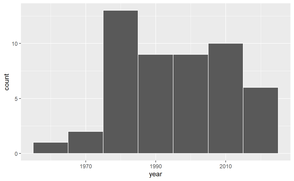
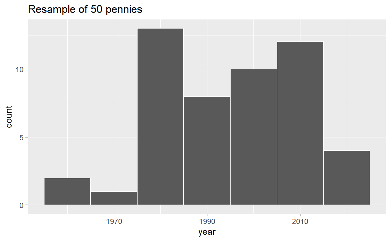
pennies_resample <- tibble(
  year = c(1976, 1962, 1976, 1983, 2017, 2015, 2015, 1962, 2016, 1976, 
           2006, 1997, 1988, 2015, 2015, 1988, 2016, 1978, 1979, 1997, 
           1974, 2013, 1978, 2015, 2008, 1982, 1986, 1979, 1981, 2004, 
           2000, 1995, 1999, 2006, 1979, 2015, 1979, 1998, 1981, 2015, 
           2000, 1999, 1988, 2017, 1992, 1997, 1990, 1988, 2006, 2000)
)

ggplot(pennies_resample, aes(x = year)) +
  geom_histogram(binwidth = 10, color = "white") +
  labs(title = "Resample of 50 pennies")

ggplot(pennies_sample, aes(x = year)) +
  geom_histogram(binwidth = 10, color = "white") +
  labs(title = "Original sample of 50 pennies")

pennies_resample %>% 
  summarize(mean_year = mean(year))

# A tibble: 1 x 1
  mean_year
      <dbl>
1     1995.

moderndive::pennies_resamples

# A tibble: 1,750 x 3
# Groups:   name [35]
   replicate name     year
       <int> <chr>   <dbl>
 1         1 Arianna  1988
 2         1 Arianna  2002
 3         1 Arianna  2015
 4         1 Arianna  1998
 5         1 Arianna  1979
 6         1 Arianna  1971
 7         1 Arianna  1971
 8         1 Arianna  2015
 9         1 Arianna  1988
10         1 Arianna  1979
# ... with 1,740 more rows

resampled_means <- pennies_resamples %>% 
  group_by(name) %>% 
  summarize(mean_year = mean(year))

ggplot(resampled_means, aes(x = mean_year)) +
  geom_histogram(binwidth = 1, color = "white", boundary = 1990) +
  labs(x = "Sampled mean year")

virtual_shovel <- bowl %>% 
  rep_sample_n(size = 50)

virtual_resample <- pennies_sample %>% 
  rep_sample_n(size = 50, replace = TRUE)

virtual_resample %>% 
  summarize(resample_mean = mean(year))

# A tibble: 1 x 2
  replicate resample_mean
      <int>         <dbl>
1         1         1997.

virtual_resamples <- pennies_sample %>% 
  rep_sample_n(size = 50, replace = TRUE, reps = 35)

virtual_resampled_means <- virtual_resamples %>% 
  group_by(replicate) %>% 
  summarize(mean_year = mean(year))

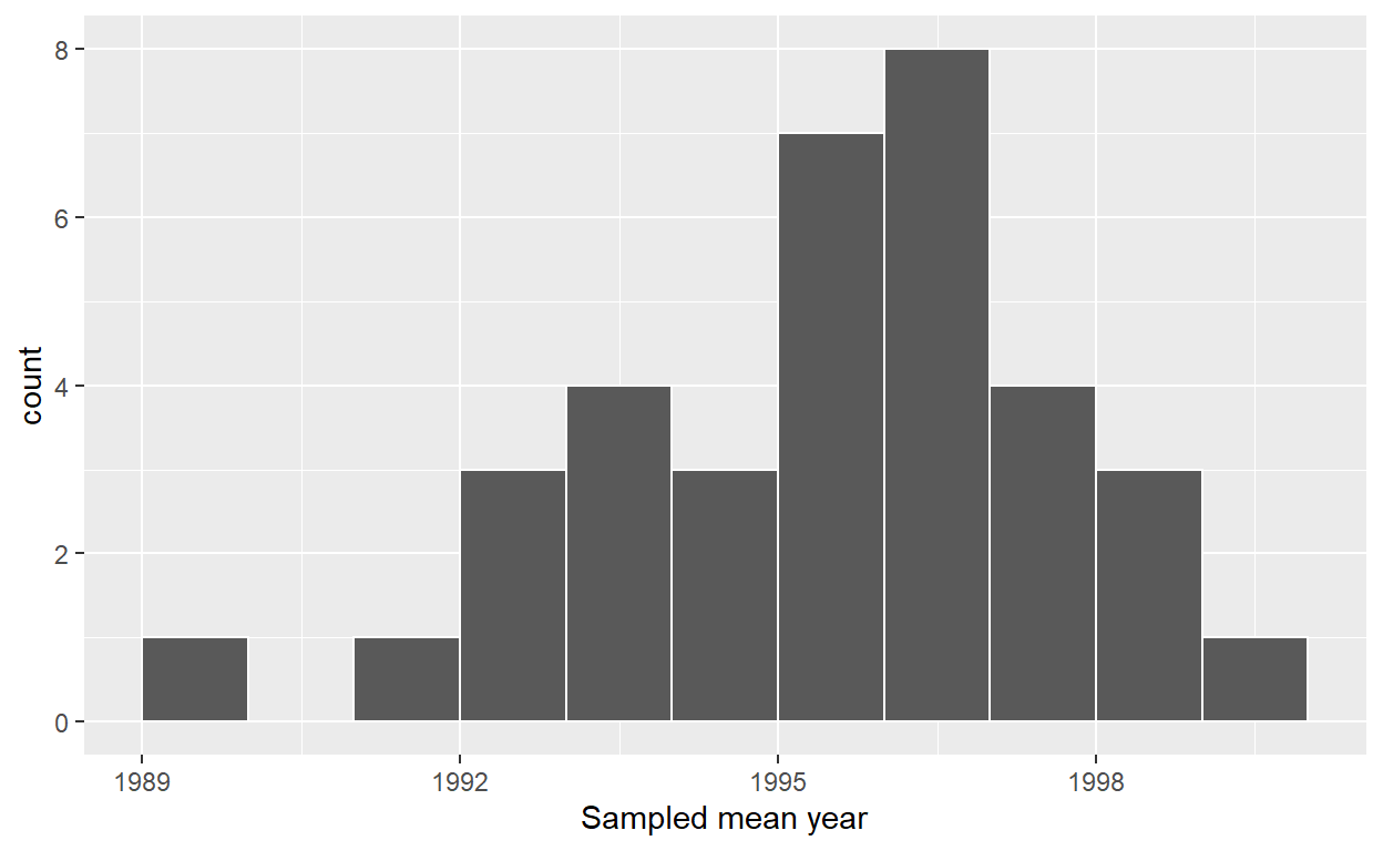
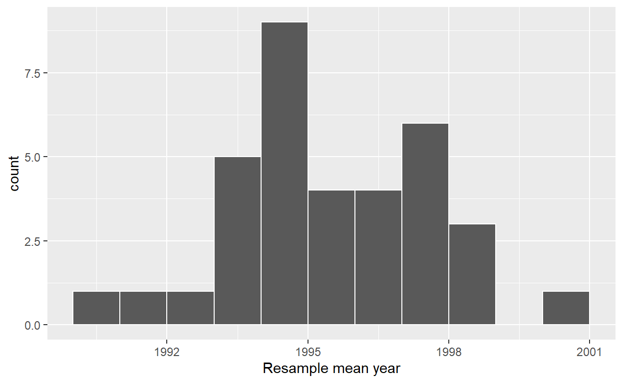
ggplot(virtual_resampled_means, aes(x = mean_year)) +
  geom_histogram(binwidth = 1, color = "white", boundary = 1990) +
  labs(x = "Resample mean year")

Repeat resampling 1000 times

virtual_resamples <- pennies_sample %>% 
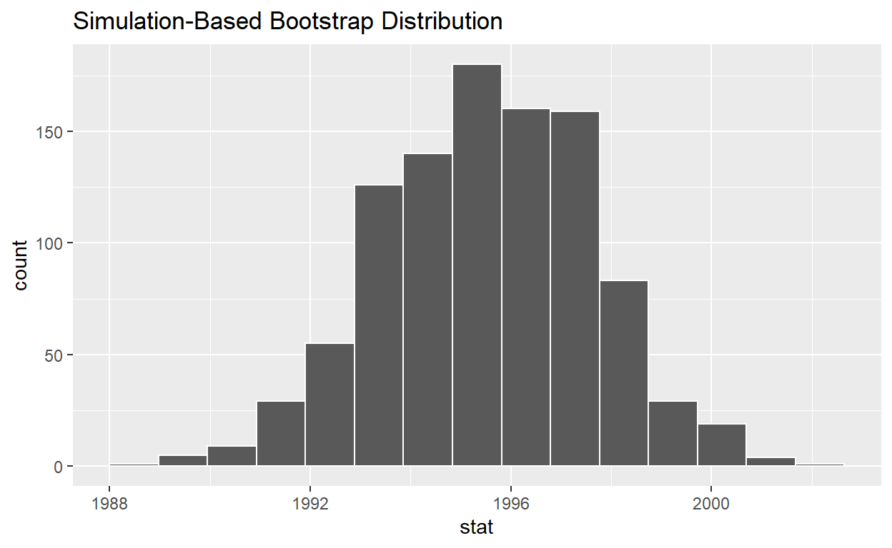
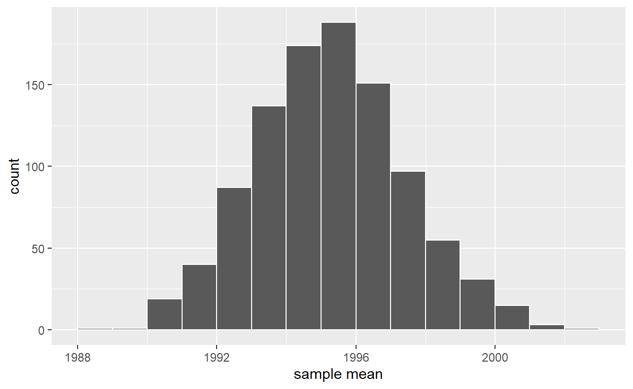
  rep_sample_n(size = 50, replace = TRUE, reps = 1000)

Compute 1000 sample means

virtual_resampled_means <- virtual_resamples %>% 
  group_by(replicate) %>% 
  summarize(mean_year = mean(year))

virtual_resampled_means <- pennies_sample %>% 
  rep_sample_n(size = 50, replace = TRUE, reps = 1000) %>% 
  group_by(replicate) %>% 
  summarize(mean_year = mean(year))

ggplot(virtual_resampled_means, aes(x = mean_year)) +
  geom_histogram(binwidth = 1, color = "white", boundary = 1990) +
  labs(x = "sample mean")

virtual_resampled_means %>% 
  summarize(mean_of_means = mean(mean_year))

# A tibble: 1 x 1
  mean_of_means
          <dbl>
1         1995.

virtual_resampled_means %>% 
  summarize(SE = sd(mean_year))

# A tibble: 1 x 1
     SE
  <dbl>
1  2.15

pennies_sample %>% 
  rep_sample_n(size = 50, replace = TRUE, reps = 1000)

# A tibble: 50,000 x 3
# Groups:   replicate [1,000]
   replicate    ID  year
       <int> <int> <dbl>
 1         1    38  1999
 2         1    47  1982
 3         1    10  2000
 4         1    12  1995
 5         1    12  1995
 6         1    50  2017
 7         1    24  2017
 8         1     3  2017
 9         1    26  1979
10         1    15  1974
# ... with 49,990 more rows

pennies_sample %>% 
  rep_sample_n(size = 50, replace = TRUE, reps = 1000) %>% 
  group_by(replicate)

# A tibble: 50,000 x 3
# Groups:   replicate [1,000]
   replicate    ID  year
       <int> <int> <dbl>
 1         1    12  1995
 2         1    23  1998
 3         1     6  1983
 4         1    49  2006
 5         1    33  1979
 6         1    10  2000
 7         1    27  1993
 8         1    34  1985
 9         1    35  1985
10         1    43  2018
# ... with 49,990 more rows

pennies_sample %>% 
  rep_sample_n(size = 50, replace = TRUE, reps = 1000) %>% 
  group_by(replicate) %>% 
  summarize(mean_year = mean(year))

# A tibble: 1,000 x 2
   replicate mean_year
       <int>     <dbl>
 1         1     1996.
 2         2     1989.
 3         3     1996.
 4         4     1995.
 5         5     1998.
 6         6     1997.
 7         7     1994.
 8         8     1995.
 9         9     1995.
10        10     1996.
# ... with 990 more rows

pennies_sample %>% 
  summarize(stat = mean(year))

# A tibble: 1 x 1
   stat
  <dbl>
1 1995.

pennies_sample %>% 
  specify(response = year) %>% 
  calculate(stat = "mean")

Response: year (numeric)
# A tibble: 1 x 1
   stat
  <dbl>
1 1995.

pennies_sample %>% 
  specify(response = year)

Response: year (numeric)
# A tibble: 50 x 1
    year
   <dbl>
 1  2002
 2  1986
 3  2017
 4  1988
 5  2008
 6  1983
 7  2008
 8  1996
 9  2004
10  2000
# ... with 40 more rows

pennies_sample %>% 
  specify(formula = year ~ NULL)

Response: year (numeric)
# A tibble: 50 x 1
    year
   <dbl>
 1  2002
 2  1986
 3  2017
 4  1988
 5  2008
 6  1983
 7  2008
 8  1996
 9  2004
10  2000
# ... with 40 more rows

pennies_sample %>% 
  specify(response = year) %>% 
  generate(reps = 1000, type = "bootstrap")

Response: year (numeric)
# A tibble: 50,000 x 2
# Groups:   replicate [1,000]
   replicate  year
       <int> <dbl>
 1         1  2004
 2         1  1971
 3         1  1996
 4         1  1985
 5         1  2006
 6         1  1996
 7         1  2015
 8         1  1962
 9         1  2017
10         1  1985
# ... with 49,990 more rows

bootstrap_distribution <- pennies_sample %>% 
  specify(response = year) %>% 
  generate(reps = 1000) %>% 
  calculate(stat = "mean")

visualize(bootstrap_distribution)

percentile_ci <- bootstrap_distribution %>% 
  get_confidence_interval(level = 0.95, type = "percentile")

visualize(bootstrap_distribution) + 
  shade_confidence_interval(endpoints = percentile_ci)

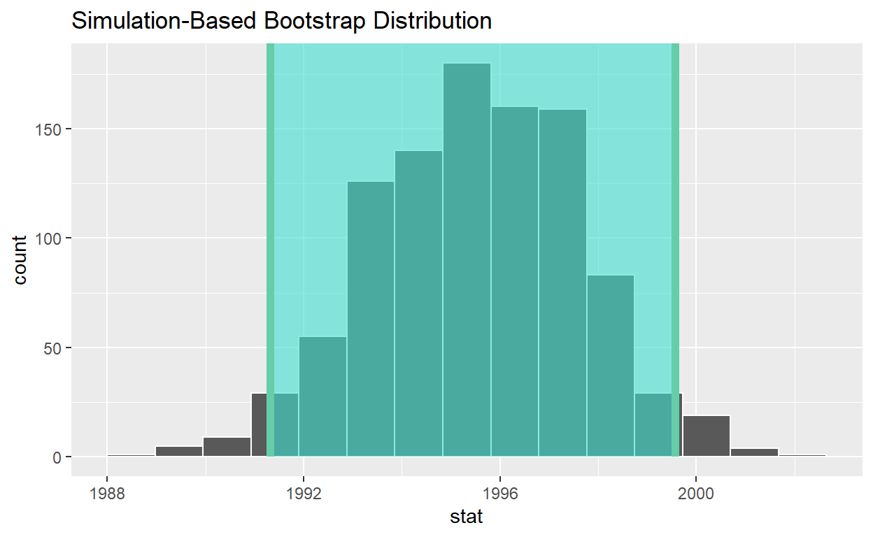
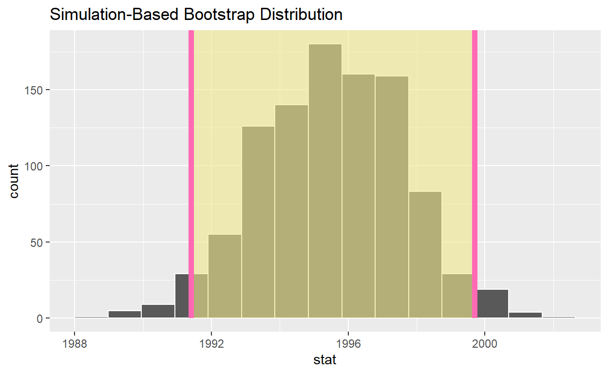
visualize(bootstrap_distribution) + 
  shade_ci(endpoints = percentile_ci, color = "hotpink", fill = "khaki")

standard_error_ci <- bootstrap_distribution %>% 
  get_confidence_interval(type = "se", point_estimate = x_bar)

visualize(bootstrap_distribution) + 
  shade_confidence_interval(endpoints = standard_error_ci)

bowl %>% 
  summarize(p_red = mean(color == "red"))

# A tibble: 1 x 1
  p_red
  <dbl>
1 0.375

moderndive::bowl_sample_1

# A tibble: 50 x 1
   color
   <chr>
 1 white
 2 white
 3 red  
 4 red  
 5 white
 6 white
 7 red  
 8 white
 9 white
10 white
# ... with 40 more rows

bowl_sample_1 %>% 
  specify(response = color, success = "red")

Response: color (factor)
# A tibble: 50 x 1
   color
   <fct>
 1 white
 2 white
 3 red  
 4 red  
 5 white
 6 white
 7 red  
 8 white
 9 white
10 white
# ... with 40 more rows

bowl_sample_1 %>% 
  specify(response = color, success = "red") %>% 
  generate(reps = 1000, type = "bootstrap")

Response: color (factor)
# A tibble: 50,000 x 2
# Groups:   replicate [1,000]
   replicate color
       <int> <fct>
 1         1 white
 2         1 white
 3         1 red  
 4         1 red  
 5         1 white
 6         1 white
 7         1 white
 8         1 red  
 9         1 white
10         1 red  
# ... with 49,990 more rows

sample_1_bootstrap <- bowl_sample_1 %>% 
  specify(response = color, success = "red") %>% 
  generate(reps = 1000, type = "bootstrap") %>% 
  calculate(stat = "prop")

percentile_ci_1 <- sample_1_bootstrap %>% 
  get_confidence_interval(level = 0.95, type = "percentile")

sample_1_bootstrap %>% 
  visualize(bins = 15) + 
  shade_confidence_interval(endpoints = percentile_ci_1) +
  geom_vline(xintercept = 0.42, linetype = "dashed")

bowl_sample_2 <- bowl %>% rep_sample_n(size = 50)

sample_2_bootstrap <- bowl_sample_2 %>% 
  specify(response = color, 
          success = "red") %>% 
  generate(reps = 1000, 
           type = "bootstrap") %>% 
  calculate(stat = "prop")

percentile_ci_2 <- sample_2_bootstrap %>% 
  get_confidence_interval(level = 0.95, type = "percentile")

moderndive::mythbusters_yawn

# A tibble: 50 x 3
    subj group   yawn 
   <int> <chr>   <chr>
 1     1 seed    yes  
 2     2 control yes  
 3     3 seed    no   
 4     4 seed    yes  
 5     5 seed    no   
 6     6 control no   
 7     7 seed    yes  
 8     8 control no   
 9     9 control no   
10    10 seed    no   
# ... with 40 more rows

mythbusters_yawn %>% 
  group_by(group, yawn) %>% 
  summarize(count = n())

# A tibble: 4 x 3
# Groups:   group [2]
  group   yawn  count
  <chr>   <chr> <int>
1 control no       12
2 control yes       4
3 seed    no       24
4 seed    yes      10

mythbusters_yawn %>% 
  specify(formula = yawn ~ group, success = "yes")

Response: yawn (factor)
Explanatory: group (factor)
# A tibble: 50 x 2
   yawn  group  
   <fct> <fct>  
 1 yes   seed   
 2 yes   control
 3 no    seed   
 4 yes   seed   
 5 no    seed   
 6 no    control
 7 yes   seed   
 8 no    control
 9 no    control
10 no    seed   
# ... with 40 more rows

first_six_rows <- head(mythbusters_yawn)

first_six_rows %>% 
  sample_n(size = 6, replace = TRUE)

# A tibble: 6 x 3
   subj group   yawn 
  <int> <chr>   <chr>
1     3 seed    no   
2     2 control yes  
3     2 control yes  
4     5 seed    no   
5     2 control yes  
6     1 seed    yes

mythbusters_yawn %>% 
  specify(formula = yawn ~ group, success = "yes") %>% 
  generate(reps = 1000, type = "bootstrap")

Response: yawn (factor)
Explanatory: group (factor)
# A tibble: 50,000 x 3
# Groups:   replicate [1,000]
   replicate yawn  group  
       <int> <fct> <fct>  
 1         1 yes   seed   
 2         1 no    control
 3         1 no    seed   
 4         1 no    seed   
 5         1 no    seed   
 6         1 no    seed   
 7         1 yes   seed   
 8         1 yes   seed   
 9         1 no    seed   
10         1 no    control
# ... with 49,990 more rows

mythbusters_yawn %>% 
  specify(formula = yawn ~ group, success = "yes") %>% 
  generate(reps = 1000, type = "bootstrap") %>% 
  calculate(stat = "diff in props")

Response: yawn (factor)
Explanatory: group (factor)
# A tibble: 1,000 x 2
   replicate    stat
       <int>   <dbl>
 1         1 -0.189 
 2         2 -0.373 
 3         3  0.0517
 4         4  0.0333
 5         5 -0.0921
 6         6  0.0676
 7         7  0.0167
 8         8 -0.0963
 9         9 -0.0164
10        10  0.190 
# ... with 990 more rows

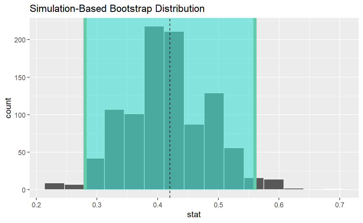
bootstrap_distribution_yawning <- mythbusters_yawn %>% 
  specify(formula = yawn ~ group, success = "yes") %>% 
  generate(reps = 1000, type = "bootstrap") %>% 
  calculate(stat = "diff in props", order = c("seed", "control"))

visualize(bootstrap_distribution_yawning) +
  geom_vline(xintercept = 0)

bootstrap_distribution_yawning %>% 
  get_confidence_interval(type = "percentile", level = 0.95)

# A tibble: 1 x 2
  lower_ci upper_ci
     <dbl>    <dbl>
1   -0.221    0.295

obs_diff_in_props <- mythbusters_yawn %>% 
  specify(formula = yawn ~ group, success = "yes") %>% 
  # generate(reps = 1000, type = "bootstrap") %>% 
  calculate(stat = "diff in props", order = c("seed", "control"))

myth_ci_se <- bootstrap_distribution_yawning %>% 
  get_confidence_interval(type = "se", point_estimate = obs_diff_in_props)

myth_ci_se

# A tibble: 1 x 2
  lower_ci upper_ci
     <dbl>    <dbl>
1   -0.215    0.304

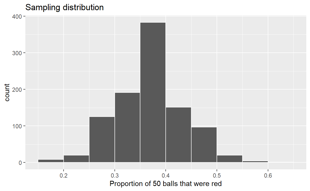
Take 1000 virtual samples of size 50 from the bowl:

virtual_samples <- bowl %>% 
  rep_sample_n(size = 50, reps = 1000)

Compute the sampling distribution of 1000 values of p-hat

sampling_distribution <- virtual_samples %>% 
  group_by(replicate) %>% 
  summarize(red = sum(color == "red")) %>% 
  mutate(prop_red = red / 50)

Visualize sampling distribution of p-hat

ggplot(sampling_distribution, aes(x = prop_red)) +
  geom_histogram(binwidth = 0.05, boundary = 0.4, color = "white") +
  labs(x = "Proportion of 50 balls that were red", 
       title = "Sampling distribution")

sampling_distribution %>% summarize(se = sd(prop_red))

# A tibble: 1 x 1
      se
   <dbl>
1 0.0658

bootstrap_distribution <- bowl_sample_1 %>% 
  specify(response = color, success = "red") %>% 
  generate(reps = 1000, type = "bootstrap") %>% 
  calculate(stat = "prop")

bootstrap_distribution %>% summarize(se = sd(stat))

# A tibble: 1 x 1
      se
   <dbl>
1 0.0711

conf_ints <- tactile_prop_red %>% 
  rename(p_hat = prop_red) %>% 
  mutate(
    n = 50,
    SE = sqrt(p_hat * (1 - p_hat) / n),
    MoE = 1.96 * SE,
    lower_ci = p_hat - MoE,
    upper_ci = p_hat + MoE
  )

Bootstrapping

Repeat resampling 1000 times

Compute 1000 sample means

Take 1000 virtual samples of size 50 from the bowl:

Compute the sampling distribution of 1000 values of p-hat

Visualize sampling distribution of p-hat