Exploratory Analysis II

To look at the different types of graphs that could describe the analytics in the forms of graphs

knitr::opts_chunk$set(echo = TRUE,
                      warning = FALSE,
                      message = FALSE)

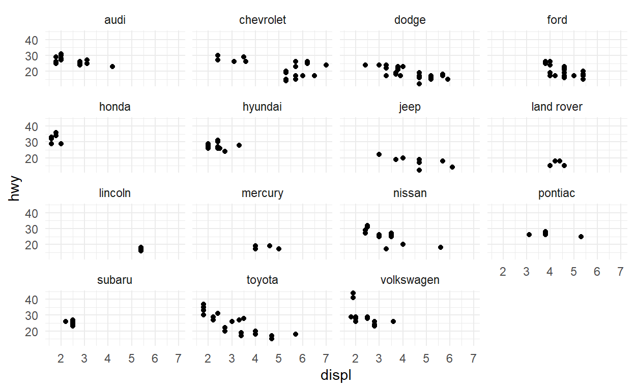
ggplot(mpg) + 
  geom_point(aes(x = displ, y = hwy)) + 
  facet_wrap(vars(manufacturer))

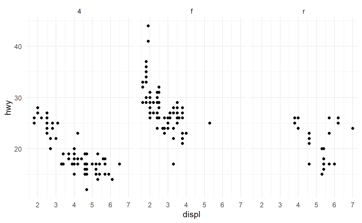
ggplot(mpg) + 
  geom_point(aes(x = displ, y = hwy)) + 
  facet_wrap(vars(drv))

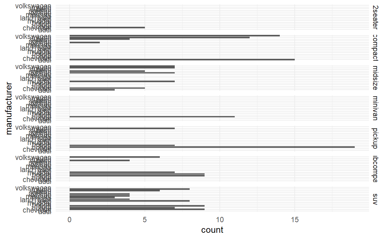
ggplot(mpg) + 
  geom_bar(aes(y = manufacturer)) + 
  facet_grid(rows = vars(class))

ggplot(mpg) + 
  geom_point(aes(x = displ, y = hwy)) + 
  facet_grid(rows = vars(year), cols = vars(drv))

ggplot(mpg) + 
  geom_point(aes(x = displ, y = hwy)) + 
  facet_wrap(vars(year, drv))

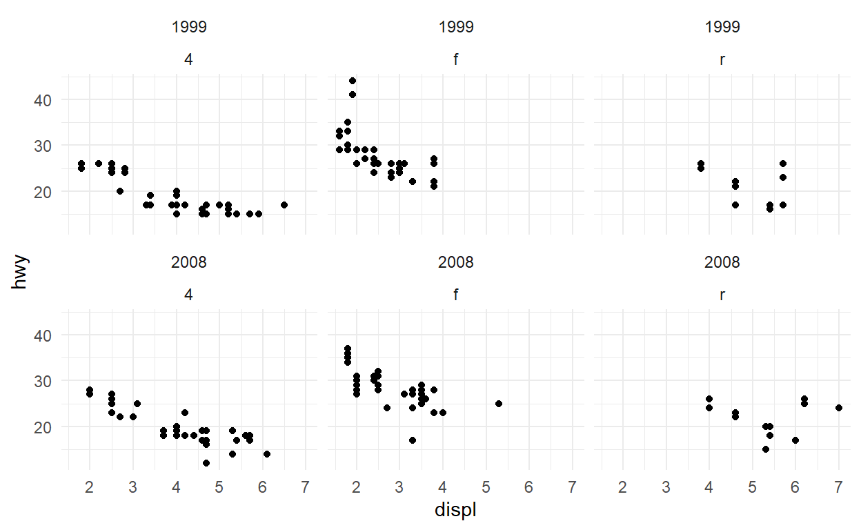
ggplot(mpg) + 
  geom_point(aes(x = displ, y = hwy)) + 
  facet_grid(rows = vars(year), cols = vars(drv))

ggplot(mpg) + 
  geom_bar(aes(y = manufacturer)) + 
  facet_grid(rows = vars(class))

ggplot(mpg) + 
  geom_point(aes(x = displ, y = hwy)) + 
  facet_grid(rows = vars(year), cols = vars(drv))

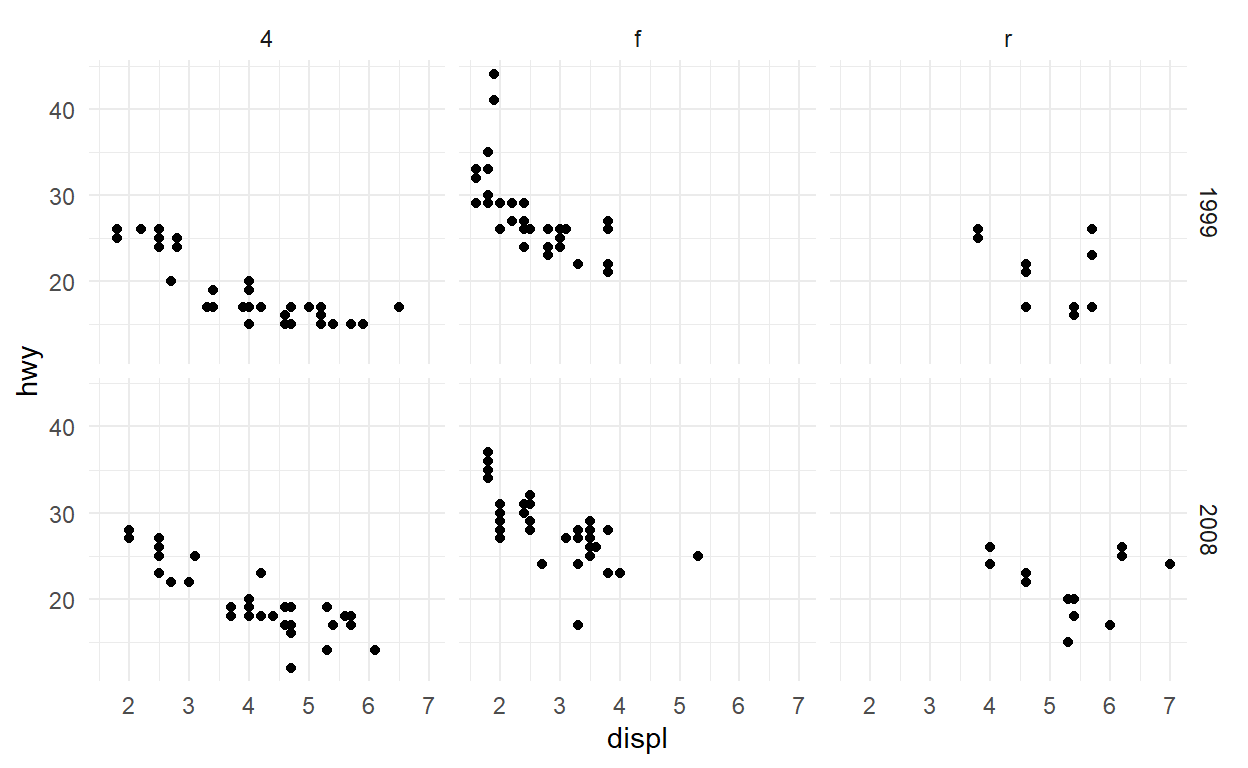
ggplot(mpg) + 
  geom_point(aes(x = displ, y = hwy)) + 
  facet_wrap(vars(year, drv))

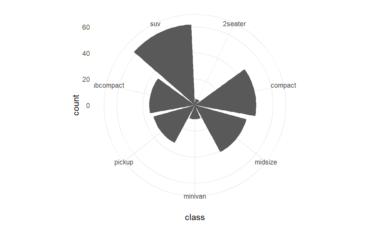
ggplot(mpg) + 
  geom_bar(aes(x = class)) + 
  coord_polar()

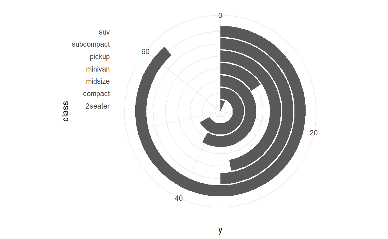
ggplot(mpg) + 
  geom_bar(aes(x = class)) + 
  coord_polar(theta = 'y') + 
  expand_limits(y = 70)

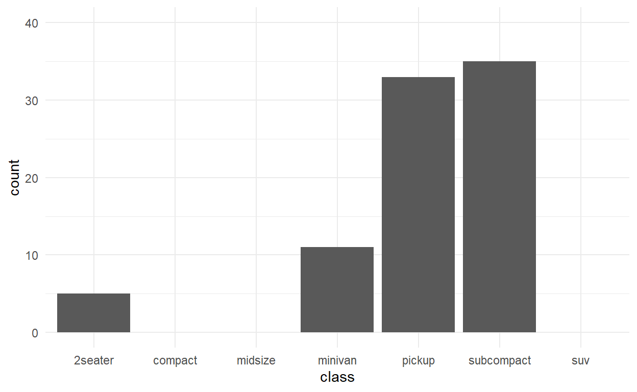
ggplot(mpg) + 
  geom_bar(aes(x = class)) + 
  scale_y_continuous(limits = c(0, 40))

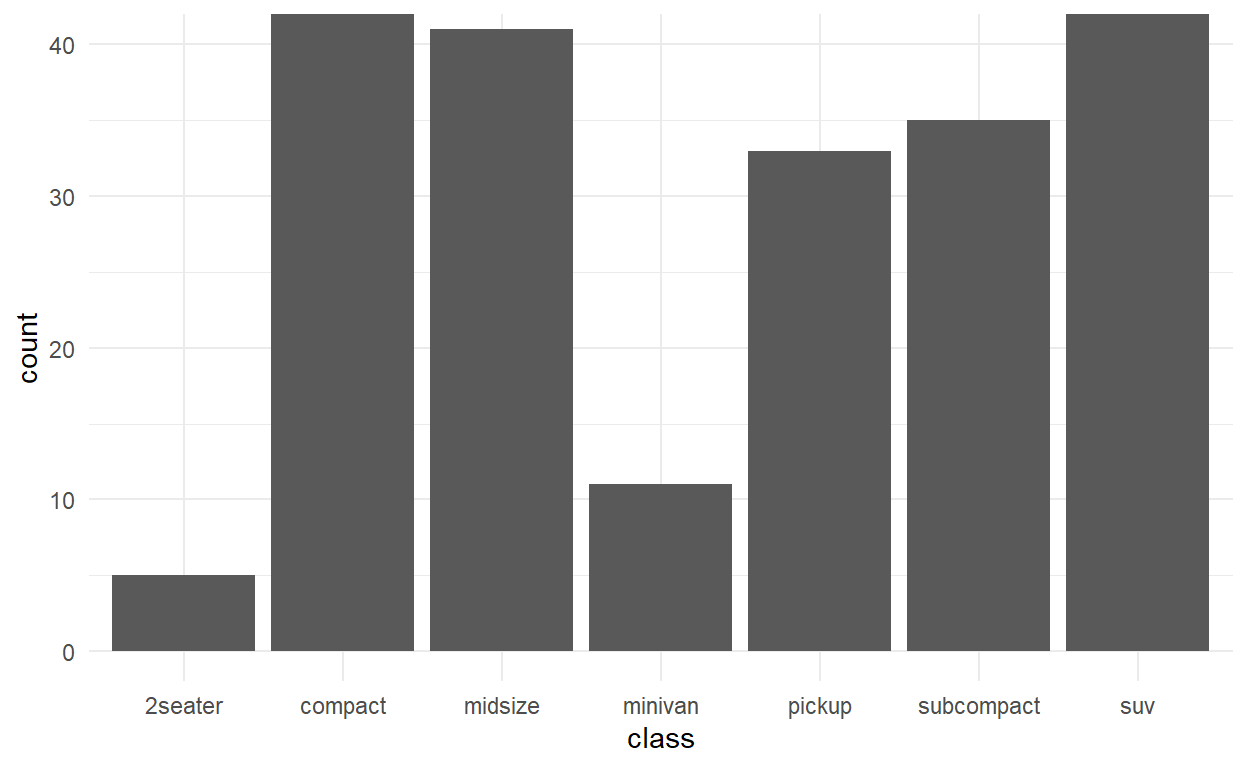
ggplot(mpg) + 
  geom_bar(aes(x = class)) + 
  coord_cartesian(ylim = c(0, 40))

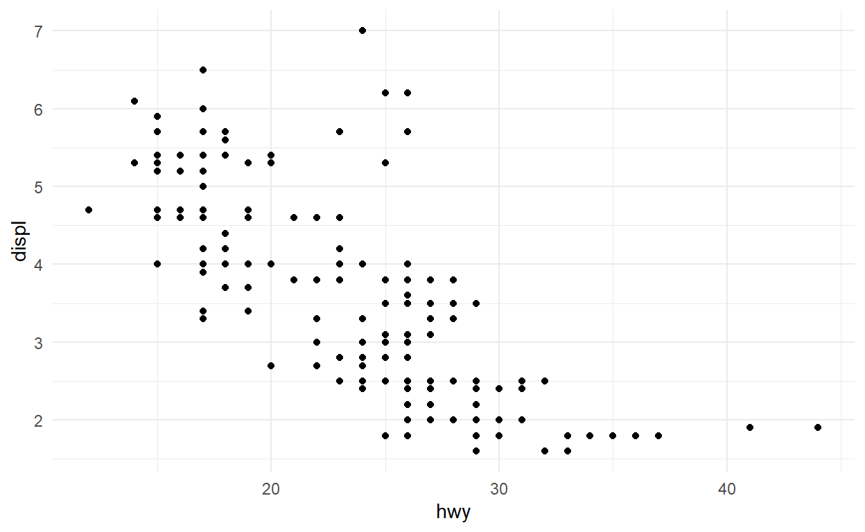
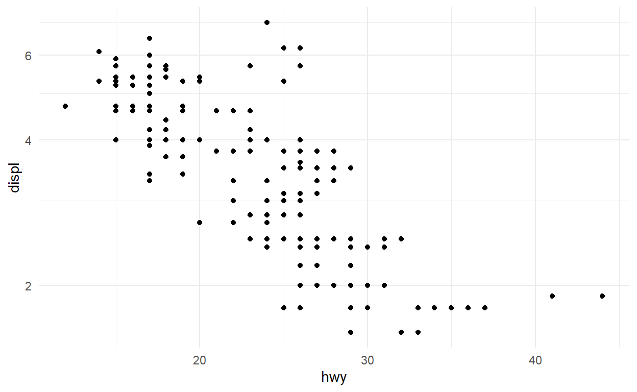
ggplot(mpg) + 
  geom_point(aes(x = hwy, y = displ))

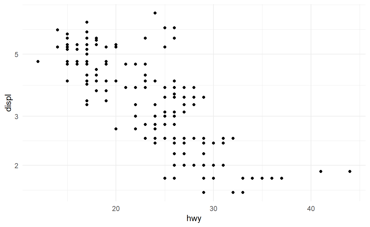
ggplot(mpg) + 
  geom_point(aes(x = hwy, y = displ)) + 
  scale_y_log10()

ggplot(mpg) + 
  geom_point(aes(x = hwy, y = displ)) + 
  coord_trans(y = "log10")

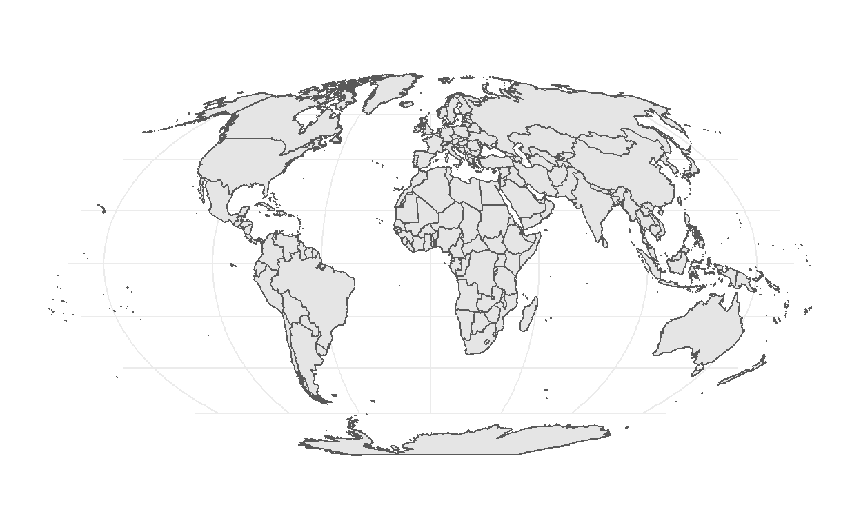
world <- sf::st_as_sf(maps::map('world', plot = FALSE, fill = TRUE))
world <- sf::st_wrap_dateline(world, 
                              options = c("WRAPDATELINE=YES", "DATELINEOFFSET=180"),
                              quiet = TRUE)
ggplot(world) + 
  geom_sf() + 
  coord_sf(crs = "+proj=moll")

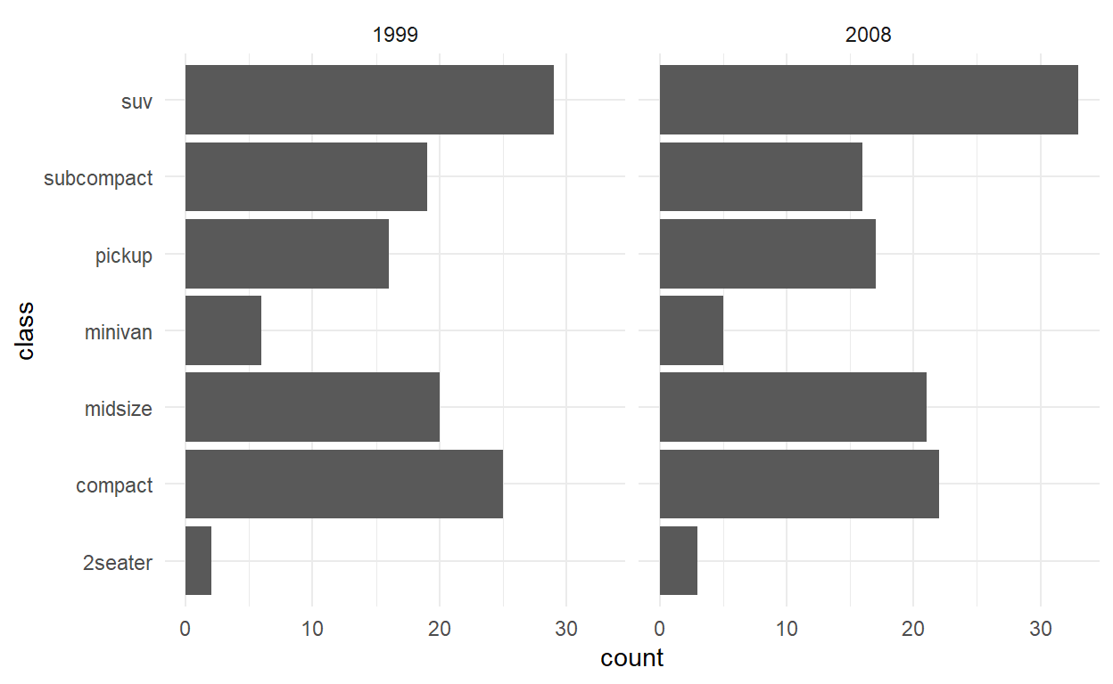
ggplot(mpg) + 
  geom_bar(aes(y = class)) + 
  facet_wrap(vars(year)) + 
  theme_minimal()

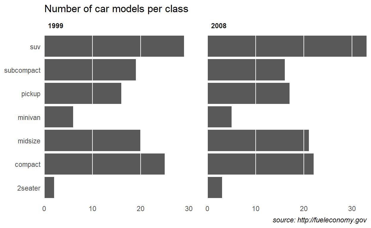
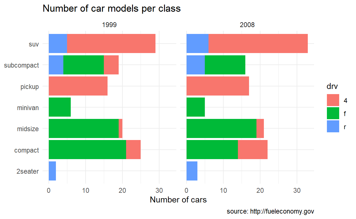
ggplot(mpg) + 
  geom_bar(aes(y = class)) + 
  facet_wrap(vars(year)) + 
  labs(title = "Number of car models per class",
       caption = "source: http://fueleconomy.gov",
       x = NULL,
       y = NULL) +
  scale_x_continuous(expand = c(0, NA)) + 
  theme_minimal() + 
  theme(
    text = element_text('Avenir Next Condensed'),
    strip.text = element_text(face = 'bold', hjust = 0),
    plot.caption = element_text(face = 'italic'),
    panel.grid.major = element_line('white', size = 0.5),
    panel.grid.minor = element_blank(),
    panel.grid.major.y = element_blank(),
    panel.ontop = TRUE
  )

ggplot(mpg) + 
  geom_bar(aes(y = class, fill = drv)) + 
  facet_wrap(vars(year)) + 
  labs(title = "Number of car models per class",
       caption = "source: http://fueleconomy.gov",
       x = 'Number of cars',
       y = NULL)

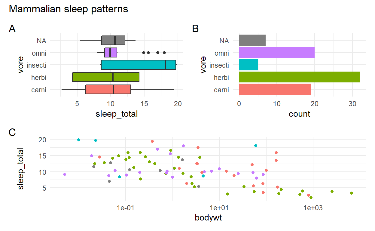
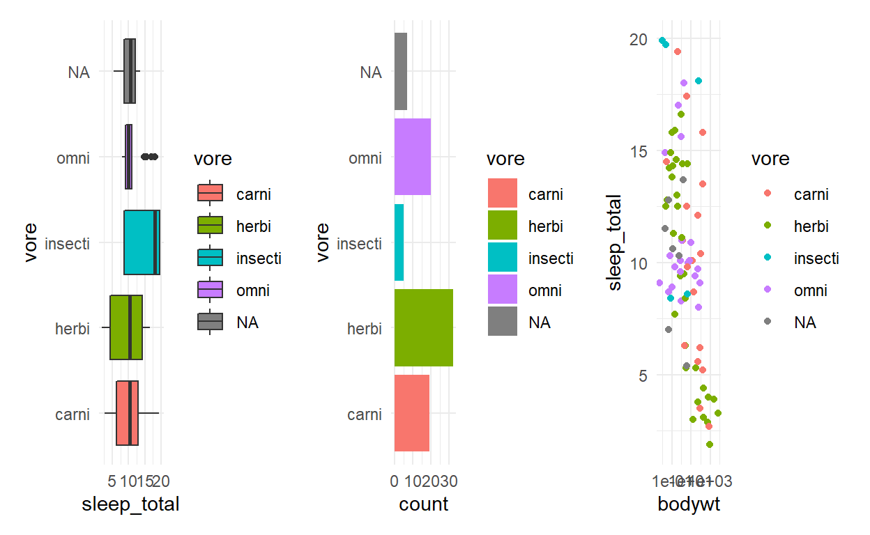
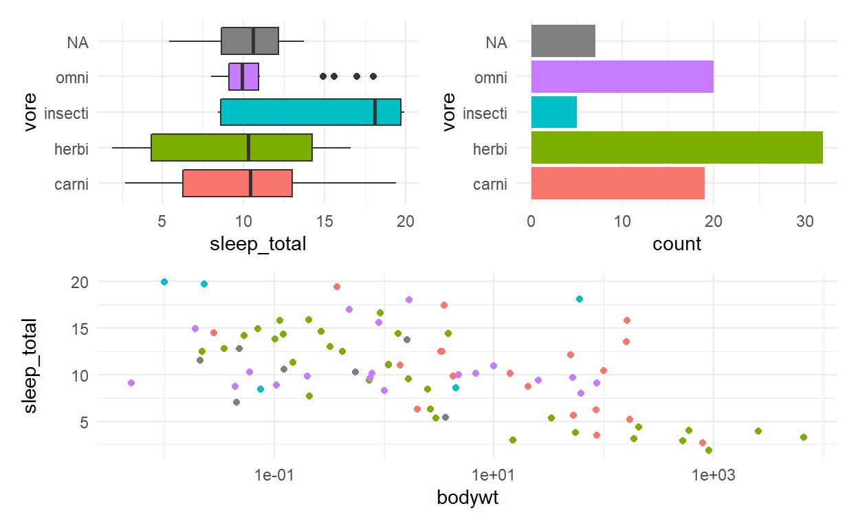
p1 <- ggplot(msleep) + 
  geom_boxplot(aes(x = sleep_total, y = vore, fill = vore))

p2 <- ggplot(msleep) + 
  geom_bar(aes(y = vore, fill = vore))

p3 <- ggplot(msleep) + 
  geom_point(aes(x = bodywt, y = sleep_total, colour = vore)) + 
  scale_x_log10()

p1 + p2 + p3

(p1 | p2) / 
   p3

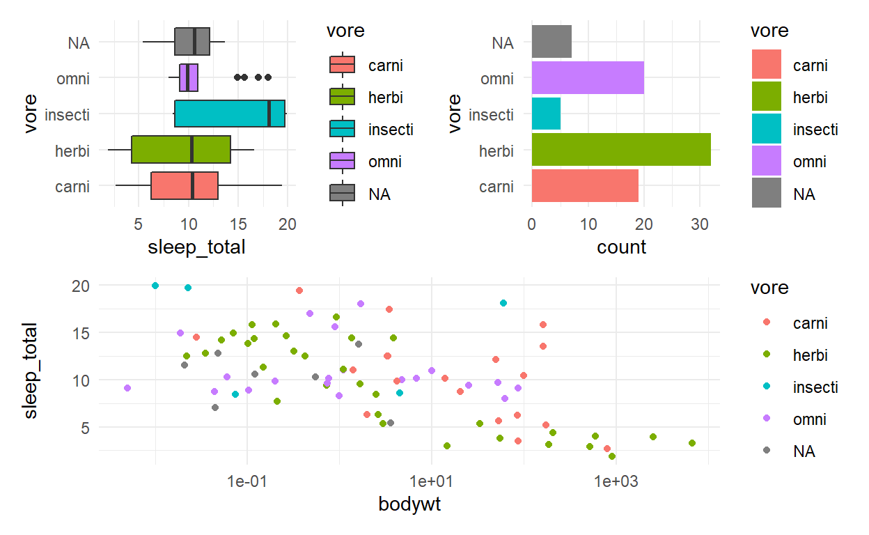
p_all <- (p1 | p2) / 
            p3
p_all + plot_layout(guides = 'collect')

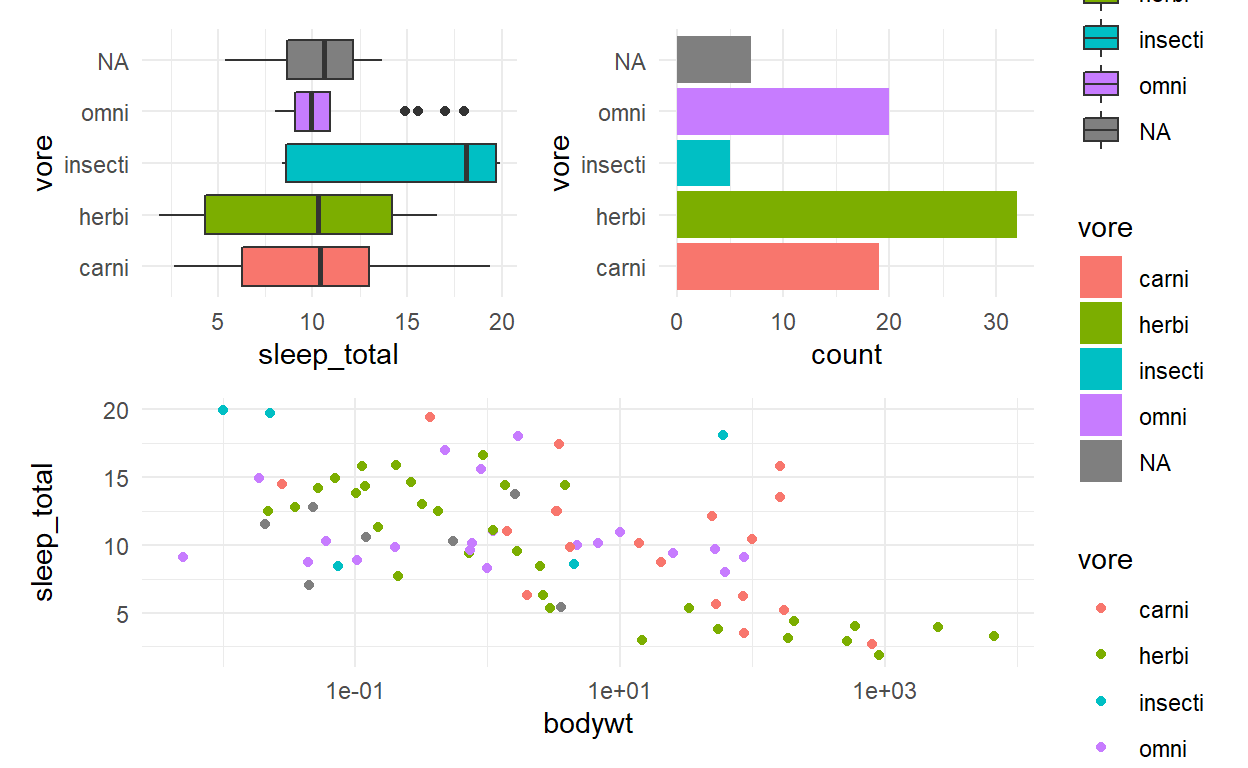
p_all & theme(legend.position = 'none')

p_all <- p_all & theme(legend.position = 'none')
p_all + plot_annotation(
  title = 'Mammalian sleep patterns',
  tag_levels = 'A'
)