Reading and writing data

1. Load the R packages we will use

library(tidyverse)
library(here)
library(janitor)
library(skimr)

2. Download \(CO_2\) emissions per capita from [Our World in Data] (https://ourworldindata.org/co2/country/united-states?country=~USA#per-capita-how-much-co2-does-the-average-person-emit) into the directory for this post.

3. Assign the location of the file to file_csv. The data should be in the same directory as this file. Read the data into R and assign it to emissions

file_csv <- here ("_posts" , 
                  "2022-02-22-reading-and-writing-data",
                  "co-emissions-per-capita.csv" )

emissions <- read_csv(file_csv)

4. Show the first 10 rows (observations of) emissions

emissions

# A tibble: 23,307 x 4
   Entity      Code   Year `Annual CO2 emissions (per capita)`
   <chr>       <chr> <dbl>                               <dbl>
 1 Afghanistan AFG    1949                              0.0019
 2 Afghanistan AFG    1950                              0.0109
 3 Afghanistan AFG    1951                              0.0117
 4 Afghanistan AFG    1952                              0.0115
 5 Afghanistan AFG    1953                              0.0132
 6 Afghanistan AFG    1954                              0.013 
 7 Afghanistan AFG    1955                              0.0186
 8 Afghanistan AFG    1956                              0.0218
 9 Afghanistan AFG    1957                              0.0343
10 Afghanistan AFG    1958                              0.038 
# ... with 23,297 more rows

5. Start with emissions data THEN use clean_names from the janitor package to make the names easier to work with assign the output to tidy_emissions show the first 10 rows of tidy_emissions

tidy_emissions <- emissions %>% 
  clean_names()

tidy_emissions

# A tibble: 23,307 x 4
   entity      code   year annual_co2_emissions_per_capita
   <chr>       <chr> <dbl>                           <dbl>
 1 Afghanistan AFG    1949                          0.0019
 2 Afghanistan AFG    1950                          0.0109
 3 Afghanistan AFG    1951                          0.0117
 4 Afghanistan AFG    1952                          0.0115
 5 Afghanistan AFG    1953                          0.0132
 6 Afghanistan AFG    1954                          0.013 
 7 Afghanistan AFG    1955                          0.0186
 8 Afghanistan AFG    1956                          0.0218
 9 Afghanistan AFG    1957                          0.0343
10 Afghanistan AFG    1958                          0.038 
# ... with 23,297 more rows

6. Start with the tidy_emissions THEN use filter to extract rows with year == 2004 THEN use skim to calculate the descriptive statistics

tidy_emissions %>% 
  filter(year == 2004) %>% 
  skim()

Table 1: Data summary

Name	Piped data
Number of rows	229
Number of columns	4
_______________________
Column type frequency:
character	2
numeric	2
________________________
Group variables	None

Variable type: character

skim_variable	n_missing	complete_rate	min	max	empty	n_unique	whitespace
entity	0	1.00	4	32	0	229	0
code	12	0.95	3	8	0	217	0

Variable type: numeric

skim_variable	n_missing	complete_rate	mean	sd	p0	p25	p50	p75	p100	hist
year	0	1	2004.00	0.00	2004.00	2004.00	2004.00	2004.00	2004.0	▁▁▇▁▁
annual_co2_emissions_per_capita	0	1	5.43	6.99	0.02	0.83	3.23	8.45	56.7	▇▁▁▁▁

7. 12 observations have a missing code. How are these observations different? start with tidy_emissions then extract rows with year == 2004 and are missing code

tidy_emissions %>% 
  filter(year == 2004, is.na(code))

# A tibble: 12 x 4
   entity                     code   year annual_co2_emissions_per_ca~
   <chr>                      <chr> <dbl>                        <dbl>
 1 Africa                     <NA>   2004                         1.16
 2 Asia                       <NA>   2004                         2.97
 3 Asia (excl. China & India) <NA>   2004                         3.61
 4 EU-27                      <NA>   2004                         8.68
 5 EU-28                      <NA>   2004                         8.79
 6 Europe                     <NA>   2004                         8.81
 7 Europe (excl. EU-27)       <NA>   2004                         8.96
 8 Europe (excl. EU-28)       <NA>   2004                         8.80
 9 North America              <NA>   2004                        14.5 
10 North America (excl. USA)  <NA>   2004                         5.53
11 Oceania                    <NA>   2004                        13.2 
12 South America              <NA>   2004                         2.36

8. start with tidy_emissions THEN use filter to extract rows with year == 2004 and without missing codes THEN use select to drop the year variable THEN use rename to change the vairable entity to country assign the output to emissions_2004

emissions_2004 <- tidy_emissions %>% 
  filter(year == 2004, !is.na(code)) %>% 
  select(-year) %>% 
  rename(country = entity)

9. which 15 countries have the highest annual_co2_emissions_per_capita ?

start with emissions_2004 THEN use slice_max to extract the 15 rows with the annual_co2_emissions_per_capita assign the output to max_15_emitters

max_15_emitters <- emissions_2004 %>% 
  slice_max(annual_co2_emissions_per_capita, n = 15)

10. which countries have the lowest annual_co2_emissions_per_capita start with emissions_2004 THEN use slice_min to extract the 15 rows with the lowest values assign the output to min_15_emitters

min_15_emitters <- emissions_2004 %>% 
  slice_min(annual_co2_emissions_per_capita, n = 15)

11. use bind_rows to bind together the max_15_emitters and min_15_emitters assign the output to max_min_15

max_min_15 <- bind_rows(max_15_emitters, min_15_emitters)

12. export max_min_15 to 3 file formats

max_min_15 %>%  write_csv("max_min_15.csv") # comma-separated values
max_min_15 %>% write_tsv("max_min_15.tsv") # tab separated
max_min_15 %>% write_delim("max_min_15.psv", delim = "|") # pipe-separated

13. read the 3 files format into R

max_min_15_csv <- read_csv("max_min_15.csv") # comma-separated values
max_min_15_tsv <- read_tsv("max_min_15.tsv") # tab separated
max_min_15_psv <- read_delim("max_min_15.psv", delim = "|") # pipe-separated

14. use setdiff to check for any differences among max_min_15_csv , max_min_15_tsv and max_min_15_psv

setdiff(max_min_15_tsv, max_min_15_psv)

# A tibble: 0 x 3
# ... with 3 variables: country <chr>, code <chr>,
#   annual_co2_emissions_per_capita <dbl>

Are there any differences? no there are no differences.

15. Reorder country in max_min_15 for plotting and assign to max_min_15_plot_data start with emissions_2019 THEN use mutate to reorder country according to annual_co2_emissions_per_capita

max_min_15_plot_data <- max_min_15 %>% 
  mutate(country = reorder(country, annual_co2_emissions_per_capita))

16. Plot max_min_15_plot_data

ggplot(data = max_min_15_plot_data, 
       mapping = aes(x = annual_co2_emissions_per_capita, y = country))

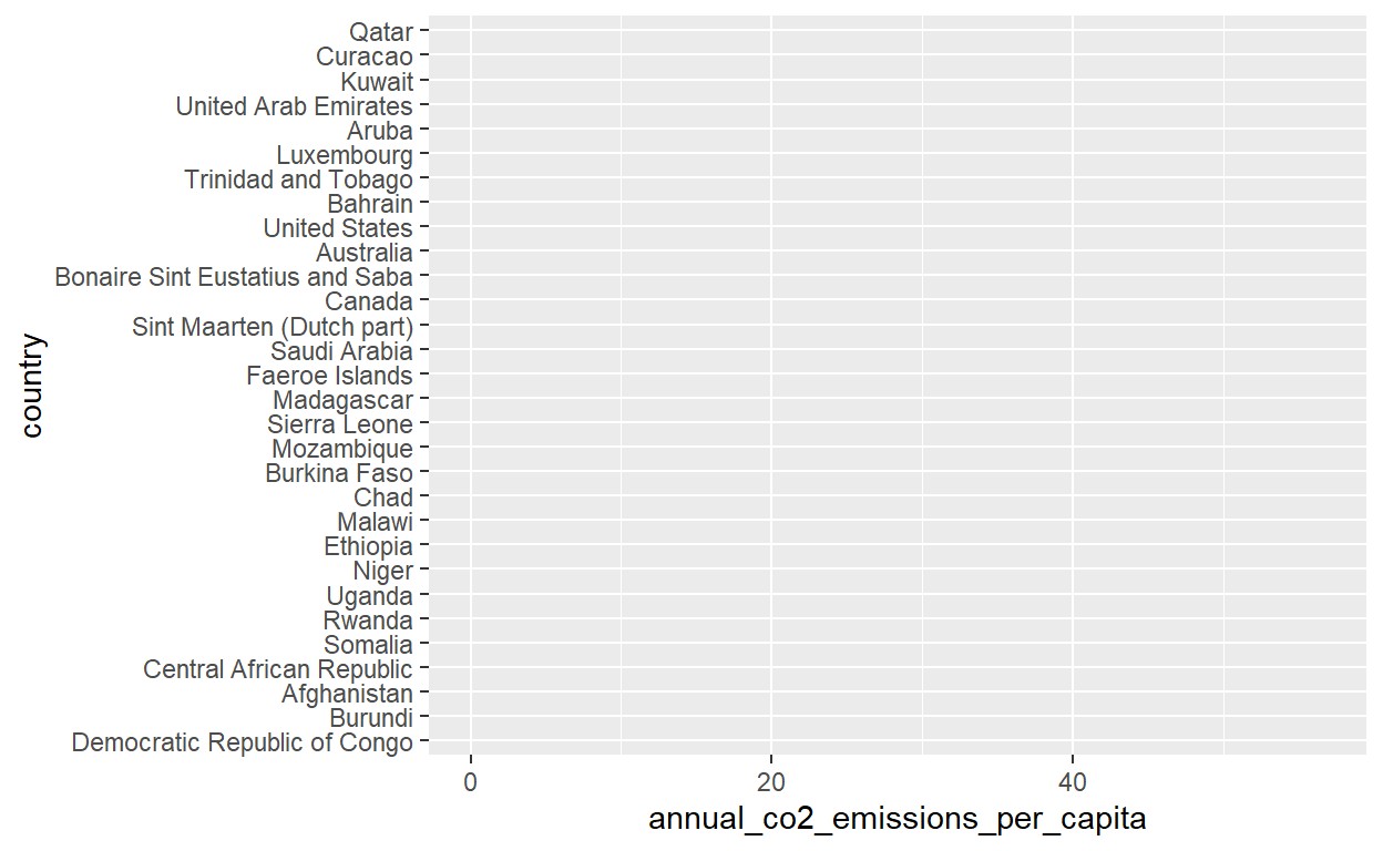
  geom_col()

geom_col: width = NULL, na.rm = FALSE
stat_identity: na.rm = FALSE
position_stack 

labs(title = "The top 15 and bottom 15 per capita CO2 emissions",
     subtitle = "for 2004",
     x = NULL,
     y = NULL)

$x
NULL

$y
NULL

$title
[1] "The top 15 and bottom 15 per capita CO2 emissions"

$subtitle
[1] "for 2004"

attr(,"class")
[1] "labels"

17. save the plot directory with this post

ggsave(filename = "preview.png",
       path = here("_posts", "2022-02-22-reading-and-writing-data"))

18. Add preview.png top yaml chunk at the top of this file

preview: preview.png